Transformed Estimators

Whenever \(x\) and \(y\) are continuous and high-dimensional, estimating mutual information may require considerable resources. Using the Data Processing Inequality (DPI), we can define a lower bound of mutual information by applying functions \(f_x\) and \(f_y\) to \(x\) and \(y\) respectively:

\[I(x;y) \ge \max_{f_y \in \mathcal{F}_y} I(x;f_y(y)) \ge \max_{f_x\in \mathcal{F}_x, f_y \in \mathcal{F}_y} I(f_x(x);f_y(y))\]

The functions \(f_x\) and \(f_y\) can be modeled via parametric neural network architectures which map structured high-dimensional data into lower-dimensional vector representations.

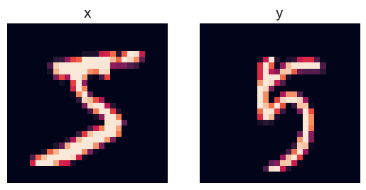
Here we will consider a simple example in which we will try to estimate mutual information between MNIST digits sampled from the same class.

import numpy as np
import matplotlib.pyplot as plt
import seaborn as sns
sns.set_style('whitegrid')
import torch

from torch.utils.data import Dataset, DataLoader
from torch import nn
from torchvision.transforms import ToTensor
from torchvision.datasets import MNIST


class PairedMNIST(Dataset):
    def __init__(self, *args, **kwargs):
        super().__init__()
        self.mnist = MNIST(*args, **kwargs)


    def __getitem__(self, idx):
        x, target = self.mnist[idx]
        idx_2 = np.random.choice(np.arange(len(dataset))[self.mnist.targets==target])
        y, target_2 = self.mnist[idx_2]
        assert target == target_2

        return {'x': x, 'y':y}

    def __len__(self):
        return self.mnist.__len__()

dataset = PairedMNIST('/data', transform=ToTensor())

# Plot an example from the dataset
f, ax = plt.subplots(1,2)
ax[0].imshow(dataset[0]['x'][0])
ax[1].imshow(dataset[0]['y'][0])
ax[0].set_title('x', fontsize=15)
ax[1].set_title('y', fontsize=15)
ax[0].axis('off')
ax[1].axis('off');

Secondly we define a simple encoder architecture which maps the images of shape \([1 \times 28 \times 28]\) into a vector of shape [z_dim].

z_dim = 16

# Simple convolutional architecture with a flattening layer
encoder = nn.Sequential(
    nn.Conv2d(1, 16, 3),
    nn.ReLU(True),
    nn.Conv2d(16, 32, 5, stride=3),
    nn.ReLU(True),
    nn.Conv2d(32, 128, 8),
    nn.ReLU(True),
    nn.Flatten(),
    nn.Linear(128, z_dim)
)

Then, we can use the TransformedMIEstimator class to estimate mutual information between the encoded images using a mutual information estimation with provides valid gradient to update the encoder. Any discriminative estimator provides a valid lower-bound, which allows us to train the encoder together with the estimator. Since the problem is symmetric in \(x\) and \(y\) we use the same encoder for both variables.

In the following example we use a simple 2-layer SMILE estimator with joint critic architecture and 8 negative samples for each pair of encoded \((f_x(x_i), f_y(y_i))\).

from torch_mist.estimators import TransformedMIEstimator, smile

transformed_estimator = TransformedMIEstimator(
    transforms={
        'x': encoder,
        'y': encoder,
    },
    base_estimator=smile(
        x_dim=z_dim,
        y_dim=z_dim,
        hidden_dims=[64, 32],
        neg_samples=32,
    )
)

transformed_estimator

TransformedMIEstimator(
  (base_estimator): SMILE(
    (ratio_estimator): JointCritic(
      (joint_net): DenseNN(
        (layers): ModuleList(
          (0): Linear(in_features=32, out_features=64, bias=True)
          (1): Linear(in_features=64, out_features=32, bias=True)
          (2): Linear(in_features=32, out_features=1, bias=True)
        )
        (f): ReLU(inplace=True)
      )
    )
    (baseline): BatchLogMeanExp()
    (neg_samples): 32
  )
  (transforms): ModuleDict(
    (x->x): Sequential(
      (0): Conv2d(1, 16, kernel_size=(3, 3), stride=(1, 1))
      (1): ReLU(inplace=True)
      (2): Conv2d(16, 32, kernel_size=(5, 5), stride=(3, 3))
      (3): ReLU(inplace=True)
      (4): Conv2d(32, 128, kernel_size=(8, 8), stride=(1, 1))
      (5): ReLU(inplace=True)
      (6): Flatten(start_dim=1, end_dim=-1)
      (7): Linear(in_features=128, out_features=16, bias=True)
    )
    (y->y): Sequential(
      (0): Conv2d(1, 16, kernel_size=(3, 3), stride=(1, 1))
      (1): ReLU(inplace=True)
      (2): Conv2d(16, 32, kernel_size=(5, 5), stride=(3, 3))
      (3): ReLU(inplace=True)
      (4): Conv2d(32, 128, kernel_size=(8, 8), stride=(1, 1))
      (5): ReLU(inplace=True)
      (6): Flatten(start_dim=1, end_dim=-1)
      (7): Linear(in_features=128, out_features=16, bias=True)
    )
  )
)

Lastly, we can train the estimator using the provided utilities and the custom dataset

from torch_mist.utils import train_mi_estimator

train_log = train_mi_estimator(
    transformed_estimator,
    train_data=dataset,
    max_epochs=10,
    verbose=True,
    lr_annealing=False,
    batch_size=128,
    num_workers=8,
)

Using the weights from the last iteration

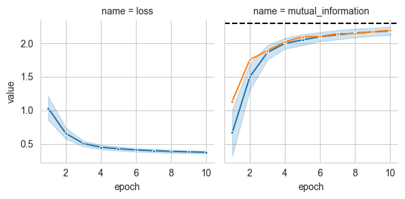
Since pairs of \(x\) and \(y\) are produced by considering data-points with the same label, we expect the mutual information value to approach \(\ln 10\).

# Plot the estimated values of mutual information over time
grid = sns.FacetGrid(train_log, col='name', hue='split')

grid.map(sns.lineplot, 'epoch', 'value', marker='.', errorbar='sd', label='estimate')
grid.axes[0,1].axhline(y=np.log(10), ls='--', color='k', label='True $I(x;y)$')

<matplotlib.lines.Line2D at 0x7fbac8941d60>

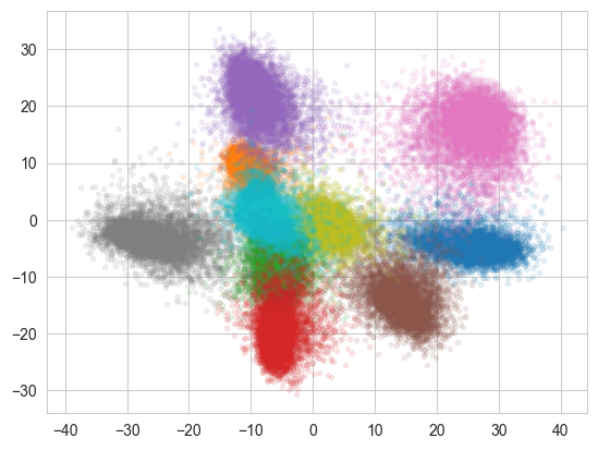
Other than mutual information estimation, this setup can be used to train encoder for dimensionality reduction. In fact, the encoder is essentially trained following the InfoMax principle:

\[\mathcal{L}^{InfoMax}(\theta) = - I(f_\theta(x),f_\theta(y))\]

Popular choices involve the use of InfoNCE, or JS (known as DeepInfoMax) for information maximization, but all discriminative estimators are supported in practice.

from sklearn.decomposition import PCA

# Compute the representation of all the images in the dataset with the trained encoder
zs = []

for data in DataLoader(dataset, batch_size=128):
    z = encoder(data['x'])
    zs.append(z)
zs = torch.cat(zs, 0).data.numpy()

# Project them to 2 dimensions using PCA
z_projected = PCA(2).fit_transform(zs)

# Plot them by label
for target in range(10):
    mask = dataset.mnist.targets==target
    plt.plot(z_projected[mask,0], z_projected[mask,1], '.', alpha=0.1)