Hybrid Mutual Information Estimators
In this example we showcase the limitation of a generative estimator (DoE) and a discriminative estimator (MINE), then show how to combine generative and generative approaches to obtain better estimates.
[1]:
import warnings
warnings.filterwarnings('ignore')
import numpy as np
import torch
import matplotlib.pyplot as plt
import seaborn as sns
from torch_mist.data.multimixture import MultivariateCorrelatedNormalMixture
from torch_mist.utils import train_mi_estimator
from torch_mist.utils.logging.metrics import compute_mean_std

import pandas as pd

sns.set_style('whitegrid')
IMG_SIZE=3
n_dim = 5


train_parameters = dict(
    max_epochs=20,
    batch_size=64,
    verbose=True,
    valid_percentage=0,
    lr_annealing=False,
    optimizer_params={'lr':5e-4},
# log the batch_loss and log_ratio methods during training and evaluation respectively
# for each one we compute the mean and standard deviation (batch-wise)
    eval_logged_methods=[
        ('log_ratio', compute_mean_std),
    ],
    train_logged_methods=[
        ('batch_loss', compute_mean_std)
    ],
    num_workers=8,
)

# Definition of the distribution
p_XY = MultivariateCorrelatedNormalMixture(n_dim=n_dim)

true_mi = p_XY.mutual_information('x','y')

p_Y_given_X = p_XY.conditional('x')
p_Y = p_XY.marginal('y')

samples = p_XY.sample([100000])
Generative Estimators: High Bias
One of the main problems of generative mutual information estimation lies in the modeling for \(q_\theta(y|x)\) and the approximation of \(H(y)\). In particular lack of flexibility for the model of \(q_\theta(y|x)\) yields under-estimation of mutual information.
We start by considering a simple difference of entropies estimator (DoE) in which \(q_\theta(y|x)\) is modeled with a conditional linear transformation of a Normal distribution, while \(r_\psi(y)\) is modeled with a parametric spline transform.
[2]:
from torch_mist.estimators import doe

estimators = {}
estimators['DoE']=doe(
    x_dim=n_dim,
    y_dim=n_dim,
    hidden_dims=[256, 128],
    conditional_transform_name='conditional_linear',
    marginal_transform_name='spline',
)


doe_log = train_mi_estimator(
    estimator=estimators['DoE'],
    train_data=samples,
    **train_parameters
)

doe_log['estimator'] = 'DoE'
log = doe_log
[Warning]: parameter hidden_dims ignored for spline.
Using the weights from the last iteration
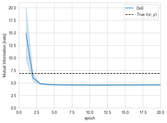
We can observe that the DoE estimator does not approach the true value of mutual information for this task. This is due to the lack of flexibility of \(q_\theta(y|x)\).
[3]:
sns.lineplot(log[log['name']=='log_ratio/mean'], x='epoch', y='value', hue='estimator', ci='sd')
plt.axhline(y=true_mi, ls='--', color='k', label='True $I(x;y)$')
plt.ylim(0,)
plt.xlim(0,20)
plt.ylabel('Mutual Information [nats]')
plt.legend();
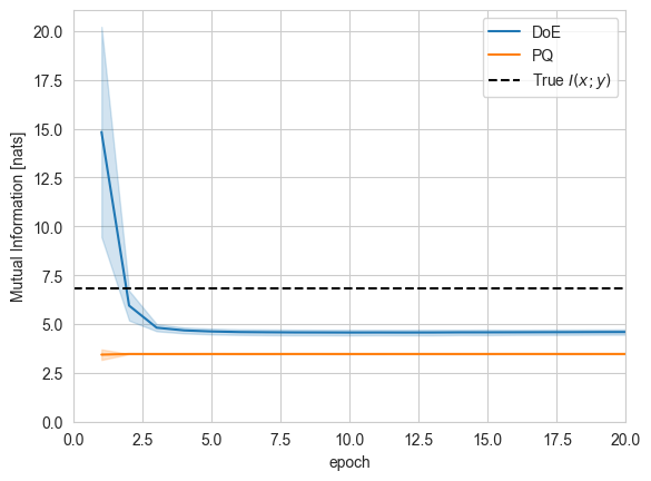
Similarly, we can instantiate and train a PQ estimator, which is based on modeling \(q_\theta(\overline{y}|x)\) and \(q_\psi(\overline{y})\) for a discretized \(\overline{y}=Q_y(y)\).
[5]:
from torch_mist.estimators import pq
from torch_mist.quantization import kmeans_quantization

# Learn a quantization function for y using K-means
quantize_y = kmeans_quantization(
    n_bins=32
)

estimators['PQ']=pq(
    x_dim=n_dim,
    quantize_y=quantize_y,
    hidden_dims=[256, 128],
)


pq_log = train_mi_estimator(
    estimator=estimators['PQ'],
    train_data=samples,
    **train_parameters
)

pq_log['estimator'] = 'PQ'
log = pd.concat([log, pq_log])
Training ClusterQuantization()
Using the weights from the last iteration
[6]:
sns.lineplot(log[log['name']=='log_ratio/mean'], x='epoch', y='value', hue='estimator', ci='sd')
plt.axhline(y=true_mi, ls='--', color='k', label='True $I(x;y)$')
plt.ylim(0,)
plt.xlim(0,20)
plt.ylabel('Mutual Information [nats]')
plt.legend();
Discriminative Estimators: High Variance
If on the one hand generative estimators are generally not powerful enough to match the true ratio, discriminative estimators are affected by high-variance. We showcase the issues of discriminative mutual information estimators by computing the mean and variance of the estimates for \(\log\frac{p(x,y)}{p(x)p(y)}\) within each training batch. For this example we use MINE mutual information estimator with a joint_critic and 1 negative sample for each positive one.
[8]:
from torch_mist.estimators import mine

estimators['MINE'] = mine(
    x_dim=n_dim,
    y_dim=n_dim,
    hidden_dims=[256, 128],
    neg_samples=1
)

mine_log = train_mi_estimator(
    estimator=estimators['MINE'],
    train_data=samples,
    **train_parameters
)

mine_log['estimator'] = 'MINE'
log = pd.concat([log, mine_log])
Using the weights from the last iteration
We can observe that the MINE estimator does not approach the true value of mutual information for this task.
[9]:
sns.lineplot(log[log['name']=='log_ratio/mean'], x='epoch', y='value', hue='estimator', ci='sd')
plt.axhline(y=true_mi, ls='--', color='k', label='True $I(x;y)$')
plt.ylim(0,)
plt.xlim(0,20)
plt.ylabel('Mutual Information [nats]')
plt.legend();
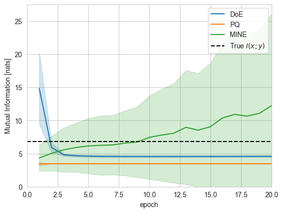
Note that the MINE estimator has considerable variance for both loss and log-ratio estimation when compared to the generative counterpart.
Hybrid mutual information estimation
By combining normalized and unnormalized distributions, we can define a more general class of estimators that can take advantage of the low variance of generative estimators and the flexibility of the discriminative approaches.
We start by defining a variational distribution \(q_\theta(x,y)\) as the product of a learnable proposal \(r_\theta(x,y)\) and an energy \(F_\theta(x,y)\):
Using the expression for \(q_\theta(x,y)\), we can derive the following estimator:
The first part of the expression is equivalent to the mutual information lower bound obtained with a generative mutual information estimation (e.g. DoE, BA, CLUB,…), while the second component has a similar expression to the discriminative approaches (e.g. MINE, NWJ, SMILE, …), with one crucial difference. When computing the partition function (last term), the samples are not drawn from the product distribution \(p(x)p(y)\), but from the proposal \(r_\theta(x,y)\) instead. Whenever \(r_\theta(x,y)\) approaches \(p(x,y)\), the variance of the estimation for the normalization constant decreases. This helps in addressing one of the main issues with discriminative estimators.
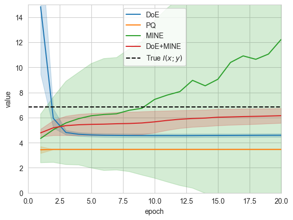
Hybrid: Difference of Entropies + MINE
One simple option for designing a suitable (normalized) proposal \(r_\theta(x,y)\) consists in modeling the conditional distribution \(r_\theta(y|x)\) instead of the entire joint:
Using this expression in the lower-bound above, we obtain:
In the following example, we will use the trained DoE estimator to approximate the generative component, and fine-tune the MINE to model the ratio between \(\log\frac{p(y|x)}{r_\theta(y|x)}\) (instead of \(\log\frac{p(y|x)}{p(y)}\) as in the original MINE estimator). This can be easily done by passing the two estimator to the HybridMIEstimator class which takes care of combining the estimates, using \(r_\theta(y|x)\) instead of \(p(y)\) to draw negative samples.
[16]:
from torch_mist.utils.freeze import freeze
from torch_mist.estimators.hybrid import ResampledHybridMIEstimator
from copy import deepcopy

# Initialize the hybrid mutual information estimator. We re-use the pre-trained DoE and MINE estimators
# Since DoE has been already trained to converge, we can freeze it to speed up the computation, which
# will focus on training the MINE estimator with negatives drawn from r(y|x) instead of p(y).
estimators['DoE+MINE'] = ResampledHybridMIEstimator(
    generative_estimator=freeze(estimators['DoE']),
    discriminative_estimator=deepcopy(estimators['MINE'])
)

hybrid_log = train_mi_estimator(
    estimator=estimators['DoE+MINE'],
    train_data=samples,
    **train_parameters
)

hybrid_log['estimator'] = 'DoE+MINE'
log = pd.concat([log, hybrid_log])
Using the weights from the last iteration
We can see that our hybrid architecture results in much more accurate estimates that slowly approach the ground-truth mutual information value. The estimates have lower variance when compared to MINE and lower bias than DoE.
[17]:
sns.lineplot(log[log['name']=='log_ratio/mean'], x='epoch', y='value', hue='estimator', errorbar='sd')
plt.axhline(y=true_mi, ls='--', color='k', label='True $I(x;y)$')
plt.ylim(0,15)
plt.xlim(0,20)
plt.legend()
[17]:
<matplotlib.legend.Legend at 0x7f946ca3f3a0>
Hybrid: Predictive Quantization and hard-negatives.
Among the various choices for the proposal \(r_\theta(x,y)\) we can consider \(p(x)(y|\overline{x})\), in which \(\overline x\) corresponds to a quantized version of \(x\). In other words, we consider \(y\) for which the corresponding \(x\) maps into the same quantization \(\overline x\):
in which \(p(x|\overline{x})\) refer to the distribution of all the \(x\) that are discretized to the same \(\overline x\).
Using this proposal, we obtain:
The first term corresponds to the PQ generative estimates, which can be seen as a difference of discrete entropies, that are easier to estimate. The second terms corresponds to a discriminative estimate in which the negatives are drown from \(p(x)p(y|\overline{x})\) instead of \(p(x)p(y)\). This is analogous to the concept of hard negative sampling, since we sample a batch of \(y\) for which the corresponding \(x\) maps to the same \(\overline x\), which we can interpret
as similar values of \(x\).
Since mutual information is symmetric, and, by convention, we defined all mutual information estimators assuming that \(y\) is lower-dimensional and easier to model, we implement a version in which we quantize \(y\) into \(\overline y\) instead, and consider \(x\) with the same \(\overline y\) as negatives. We do this by first sampling one \(\overline{y}\) then creating batches of pairs \((x_i,y_i)\) with \(y_i\) that correspond to the sampled \(\overline y\).
Note that in order to make sure that each batch contains the appropriate amount of negative samples, we make sure to sample multiple \(y\) that map to the same \(\overline y\) in the same batch. With batch size \(N\) and \(M\) as the number of negatives, we sample batches as follows:
Sample \(K=N//(M+1)\) quantized \(y\) : \([\overline y_i]_{i=1}^K\sim p(\overline{y})\)
Sample \(M\) pairs \((x_{ij}, y_{ij})\) for which \(Q(y_{ij})=\overline{y}_i\) for each \(\overline{y}_i\) sampled in the previous step: \([(x_{ij},y_{ij})]_{j=1}^M \sim p(x,y|\overline{y})\)
This procedure results in batches of size \(N\) in which each pair has \(M\) negatives sampled from \(p(x,y|\overline{y})\) that can be contrasted against, and it is integrated in the train_mi_estimator function, which takes care of creating/modifying the data-loader.
[18]:
from torch_mist.estimators import hybrid_pq

# We define the hybrid PQ+MINE estimator using the same MINE discriminative estimator trained before as a starting point
estimators['PQ+MINE'] = hybrid_pq(
    quantize_y=quantize_y,
    x_dim=n_dim,
    hidden_dims=[256, 128],
    discriminative_estimator=deepcopy(estimators['MINE'])
)

# Note that the train_mi_estimator internally creates data-loader to sample batches of (x_i, y_i)
# for which Q(y_i) is the same for the whole batch
hybrid_log = train_mi_estimator(
    estimator=estimators['PQ+MINE'],
    train_data=samples,
    **train_parameters
)

hybrid_log['estimator'] = 'PQ+MINE'
log = pd.concat([log, hybrid_log])
Using the weights from the last iteration
[20]:
sns.lineplot(log[log['name']=='log_ratio/mean'], x='epoch', y='value', hue='estimator', errorbar='sd')
plt.axhline(y=true_mi, ls='--', color='k', label='True $I(x;y)$')
plt.ylim(0,15)
plt.xlim(0,20)
plt.legend()
[20]:
<matplotlib.legend.Legend at 0x7f940a05e6d0>
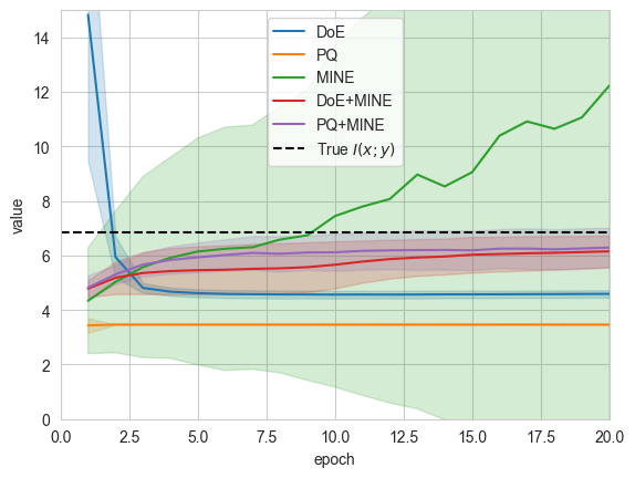
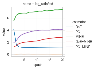
The variance of the hybrid estimators is indeed lower than MINE. This is because the variance for the estimation of the log-partition function grows as \(e^{KL(p(x,y)||r_\theta(x,y))}\), and the proposal \(r_\theta(x,y)\) used by the hybrid estimator is closer to the joint \(p(x,y)\) than the product of the marginal \(p(x)p(y)\).
As a result, the energy \(F(x,y)\) needs to do “less work” to transform \(p(x)p(y|\overline{x})\) into \(p(x,y)\).
[26]:
grid = sns.FacetGrid(log[log['name']=='log_ratio/std'], col='name', hue='estimator', sharey=False, sharex=True)
grid.map(sns.lineplot, 'epoch', 'value', errorbar='ci')
grid.add_legend()
[26]:
<seaborn.axisgrid.FacetGrid at 0x7f946fdc8c70>
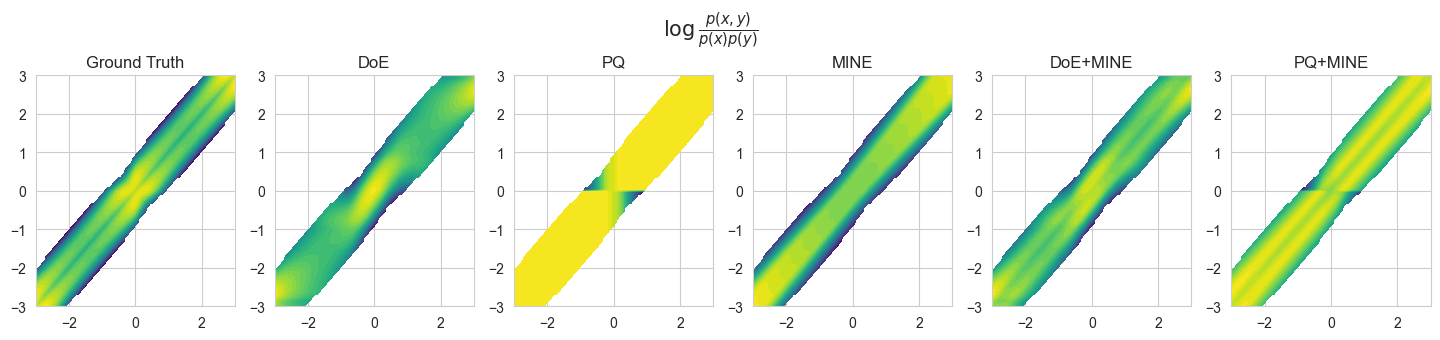
We can further showcase the differences between the estimators by plotting the modeled log-ratios.
[27]:
# We create a uniform grid to visualize the functions modeled by conditional distributions
res = 100
x_grid = torch.linspace(-3,3,res).view(1,-1,1)
y_grid = torch.linspace(-3,3, res).view(-1,1,1)
X, Y = np.meshgrid(x_grid, y_grid)

# Compute the true log-ratio log p(x,y)p(x)p(y) on the grid
log_marginal = p_XY.marginal('x').log_prob(x=x_grid)/n_dim +  p_XY.marginal('y').log_prob(y=y_grid)/n_dim
log_joint = p_XY.log_prob(x=x_grid, y=y_grid)/n_dim
# We visualize only the points for which p(x,y) > e^{-20}
mask = (log_joint>-25).data.numpy()
log_ratio = (log_joint - log_marginal).data.numpy()


f, ax = plt.subplots(
    1,1+len(estimators),
    figsize=((1+len(estimators))*IMG_SIZE, IMG_SIZE)
)

# Plot the true log-ratio
f.suptitle("$\\log \\frac{p(x,y)}{p(x)p(y)}$", fontsize=15, y=1.1)
ax[0].contourf(X, Y, log_ratio/mask, cmap='viridis', levels=40)
ax[0].set_title('Ground Truth')

for i, (name, estimator) in enumerate(estimators.items()):
    log_ratio = estimator.unnormalized_log_ratio(x_grid.repeat(res,1,n_dim), y_grid.repeat(1,res,n_dim)).data.numpy()/n_dim

    ax[i+1].contourf(X, Y, log_ratio/mask, cmap='viridis', levels=40)
    ax[i+1].set_title(name)
It is possible to use the HybridMIEstimator class to model combinations of different generative and discriminative estimators (e.g. BA+SMILE, CLUB+JS, L1Out+FLO, …).
[ ]: